Python Tutorial on Linear Regression with Batch Gradient Descent

I learn best by doing and teaching. And while Python has some excellent packages available for linear regression (like Statsmodels or Scikit-learn), I wanted to understand the intuition behind ordinary least squares (OLS) linear regression. How is the best fit found? How do you actually implement batch gradient descent? There are plenty of great explanation on gradient descent here, here and here, so my goal here is provide some insight as I implement it with Python.

This guide is primarily modeled after Andrew Ng’s excellent Machine Learning course available online for free. The programming exercises there are straight forward and intuitive, but it’s mainly in Matlab/Octave. I wanted to implement the same thing in Python with Numpy arrays.

You can also find the iPython Notebook version of this tutorial available on my Github, or in HTML format here

Packages:

Pandas for data frames and easy to read csv files
Numpy for array and matrix mathematics functions
Matplotlib for plotting

Loading the Data

Let’s start by performing a linear regression with one variable to predict profits for a food truck. The data contains 2 columns, population of a city (in 10,000s) and the profits of the food truck (in 10,000s).

data = pd.read_csv('ex1data1.txt', names = ['population', 'profit'])
print data.head()

#  population   profit
    6.1101  17.5920
    5.5277   9.1302
    8.5186  13.6620
    7.0032  11.8540
    5.8598   6.8233

Plotting the Data

plotting the data

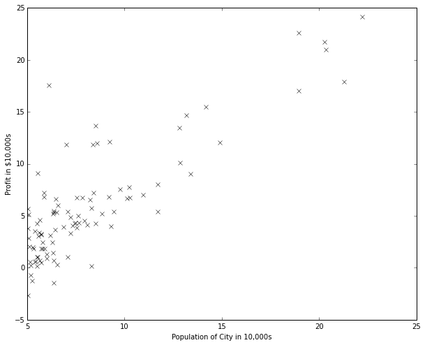
So this is what our data points look like when plotted out.

The idea of linear regression is to find a relationship between our target or dependent variable (y) and a set of explanatory variables ($x_1, x_2…$). This relationship can then be used to predict other values.

In our case with one variable, this relationship is a line defined by parameters $\beta$ and the following form: $y = \beta_0 + \beta_1x$, where $\beta_0$ is our intercept. (I chose to use $\beta$ but many literature uses $Theta$, so keep that in mind)

This can be extended to multivariable regression by extending the equation in vector form: $y=X\beta$

So how do I make the best line? In this figure, there are many possible lines. Which one is the best?

Cost Function

It turns out that to make the best line to model the data, we want to pick parameters $\beta$ that allows our predicted value to be as close to the actual value as possible. In other words, we want the distance or residual between our hypothesis $h(x)$ and y to be minimized.

So we formally define a cost function using ordinary least squares that is simply the sum of the squared distances. To find the liner regression line, we adjust our beta parameters to minimize:

$J(\beta) = \frac{1}{2m}\sum_{i=1}^m(h_\beta(x^{(i)})-y^{(i)})^2$

Again the hypothesis that we’re trying to find is given by the linear model:

$h_\beta(x) = \beta^{T}x = \beta_0 + \beta_1x_1$

And we can use batch gradient descent where each iteration performs the update

$\beta_j := \beta_j - \alpha\frac{1}{m}\sum_{i=1}^m (h_\beta(x^{(i)})-y^{(i)})x_{j}^{(i)}$

Gradient Descent?

Whoa, what’s gradient descent? And why are we updating that?

Gradient descent simply is an algorithm that makes small steps along a function to find a local minimum. We can look at a simply quadratic equation such as this one:

quadratic

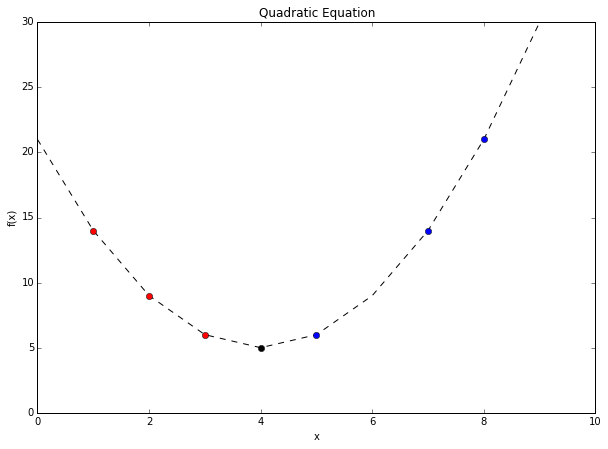
We’re trying to find the local minimum on this function. If we start at the first red dot at x = 2, we find the gradient and we move against it. In this case, the gradient is the slope. And since the slope is negative, our next attempt is further to the right. Thus bringing us closer to the minimum.

If we start at the right-most blue dot at x = 8, our gradient or slope is positive, so we move away from that by multiplying it by a -1. And it eventually makes smaller and smaller updates (as the gradient approaches 0 at the minimum) until the parameter converges at the minimum we’re looking for.

Indeed, we keep updating our parameter beta to get us closer and closer to the minimum.

$\beta_j := \beta_j - \alpha\frac{\partial}{\partial \beta_j} J(\beta)$

Where $\alpha$ is our learning rate and we find the partial differentiation of our cost function in respect to beta. I won’t derive the partial differentiation today, but it results in the formula right before this.

By adjusting alpha, we can change how quickly we converge to the minimum (at the risk of overshooting it entirely and does not converge on our local minimum)

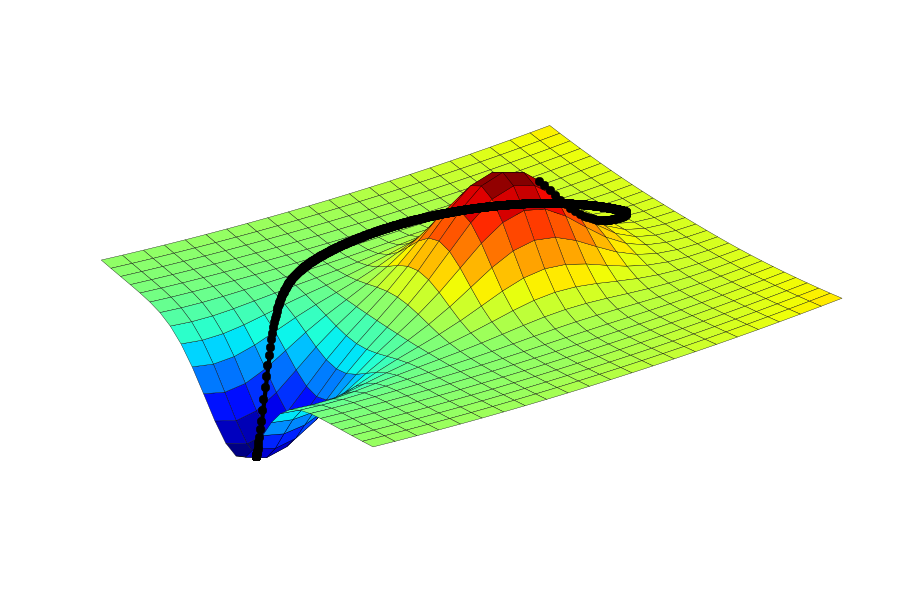
That’s in a 2 dimensional space. In a 3D space, it would be like rolling a ball down a hill to find the lowest point. I can’t picture anything above 3 dimensions, but that’s the idea.

This method is called “batch” gradient descent because we use the entire batch of points X to calculate each gradient, as opposed to stochastic gradient descent. which uses one point at a time. I’ll implement stochastic gradient descent in a future tutorial.

Python Implementation

OK, let’s try to implement this in Python. First I declare some parameters. Alpha is my learning rate, and iterations defines how many times I want to perform the update.

Then I transform the data frame holding my data into an array for simpler matrix math. And then write a function to calculate the cost function as defined above. I use np.dot for inner matrix multiplication. Here’s what it looks like:

iterations = 1500
alpha = 0.01

## Add a columns of 1s as intercept to X. This becomes the 2nd column
X_df['intercept'] = 1

## Transform to Numpy arrays for easier matrix math
## and start beta at 0, 0
X = np.array(X_df)
y = np.array(y_df).flatten()
beta = np.array([0, 0])

def cost_function(X, y, beta):
    """
    cost_function(X, y, beta) computes the cost of using beta as the
    parameter for linear regression to fit the data points in X and y
    """
    ## number of training examples
    m = len(y)

    ## Calculate the cost with the given parameters
    J = np.sum((X.dot(beta)-y)**2)/2/m

    return J

cost_function(X, y, beta)
>>> 32.07

Now, let’s implement gradient descent. Remember that long equation above? $\beta_j := \beta_j - \alpha\frac{1}{m}\sum_{i=1}^m (h_\beta(x^{(i)})-y^{(i)})x_{j}^{(i)}$

I’m going to split them into separate parts so that I can see what’s going on. Plus, I like to check my matrix dimensions to make sure that I’m doing the math in the right order. Oh and since I’m doing the math matrices now, I can exclude the summation of i terms.

Calculate hypothesis $h_\beta(x)$:
- hypothesis [97x1] = x [97x2] * beta [2x1]
Calculate loss $(h_\beta(x)-y)$:
- loss [97x1] with element-wise subtraction
Calculate gradient $(h_\beta(x)-y)x_{j}$:
- gradient [2x1] = X’ [2x97] * loss [97x1]
Update parameter beta:
- [2x1] after element-wise subtraction multiplied by a scalar
And find the cost by using cost_function()

def gradient_descent(X, y, beta, alpha, iterations):
    """
    gradient_descent() performs gradient descent to learn beta by
    taking num_iters gradient steps with learning rate alpha
    """
    cost_history = [0] * iterations

    for iteration in range(iterations):
        hypothesis = X.dot(beta)
        loss = hypothesis-y
        gradient = X.T.dot(loss)/m
        beta = beta - alpha*gradient
        cost = cost_function(X, y, beta)
        cost_history[iteration] = cost

        ## If you really want to merge everything in one line:
        # beta = beta - alpha * (X.T.dot(X.dot(beta)-y)/m)
        # cost = cost_function(X, y, beta)
        # cost_history[iteration] = cost

    return beta, cost_history

(b, c) = gradient_descent(X, y, beta, alpha, iterations)

print b
>>> [ 1.16636235 -3.63029144]

Interpretation

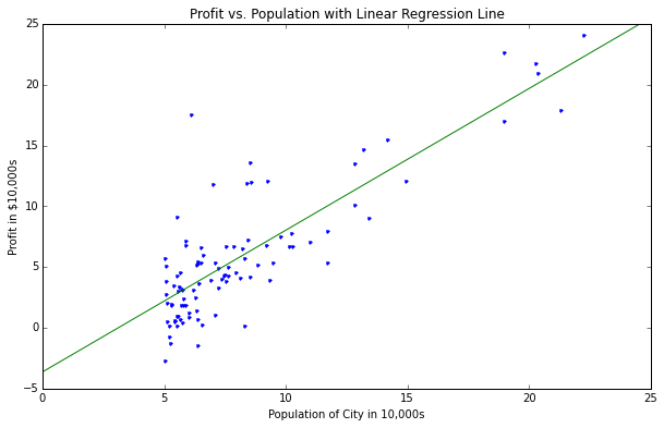
How can we interpret the beta parameters? Well $\beta_0$ is the intercept of the line in 2D. In our case, since we added the intercept column of 1s afterwards, it is actually the second column of the matrix X. So the corresponding beta is the second one. Our intercept is -3.6. Indeed, we can see on the graph with the best fit line that this is true. $\beta_0$ is then the slope of the line.

With everything put together:

linear-regression

Prediction

Now We can use our trained linear regression model to predict profits in cities of certain sizes. Let’s try 2 cities, with population of 35,000 and 70,000. Since I have my parameters defined, I can plug them in to the linear regression model: $\hat{y} = -3.603 + 1.166x$

or make them a matrix x and multiple them by beta

print np.array([3.5, 1]).dot(b)
print np.array([7, 1]).dot(b)
>>> 0.45197678677
>>> 4.53424501294

Profits are about $4,519 and $45,342 respectively.

See, gradient descent isn’t difficult to understand anymore. Of course, I glossed over some important considerations (such as learning rate and number of iterations until converging on a minumum), and they may be topics for another day, but this is the general concept.

Next up, we’ll take a look at regularization and multi-variable regression, before exploring logistic regression and other supervised learning algorithms.

Let me know if this was helpful or if you spotted any errors.

-->

Contents: