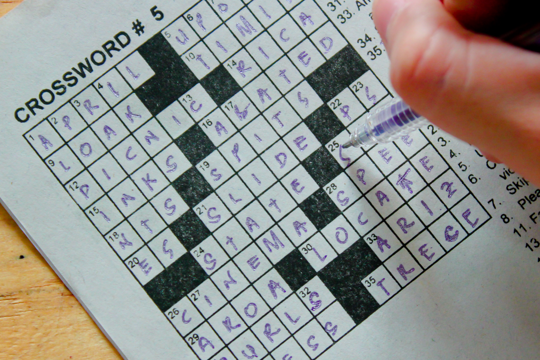
Are people “cheating” on crossword puzzles?
I’ve been solving crossword puzzles for more than 15 years now. While I don’t cheat by Googling the clues, I do allow myself to research esoteric clues on Wikipedia to learn about them. However, I can’t help but notice the growing number of websites dedicated to just crossword puzzle answers. How many people are actually searching the web for these answers? Who’s “cheating”? Can we quantify this?
Using Google Trends
Fortunately, we have an excellent resource to help us determine this: Google Trends! This is an invaluable tool in my professional career and personal musings as it tracks what people are searching for. At work, it becomes a proxy of consumer interests and brand awareness. We can measure engagement of TV advertising by assume that a percentage of viewers might be piqued by our brand’s ad and search for the brand on Google. In this case, we can see when people are searching for specific crossword puzzle clues to get the answers.
It would be helpful to understand that Google doesn’t actually show exact search volumes of specific keywords, they present a normalized index from a sampled percentage of actual searches within the timeframe of our request. Here are some more details from Google.
Example
Let’s use a clue from a crossword puzzle clue from 3/28/2019 as a demonstration:
2 Down: Subject of Hemingway’s “Death in the Afternoon”
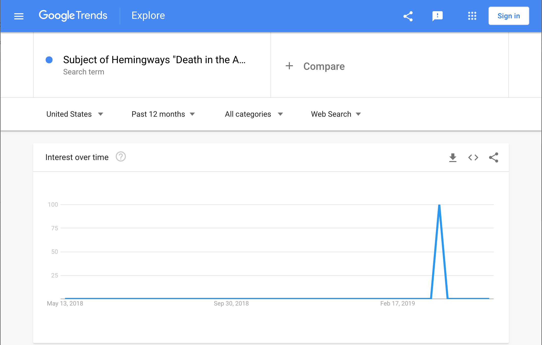
Just searching for the entire clue in Google Trends shows that indeed there was a spike of searches on the day the crossword was published!
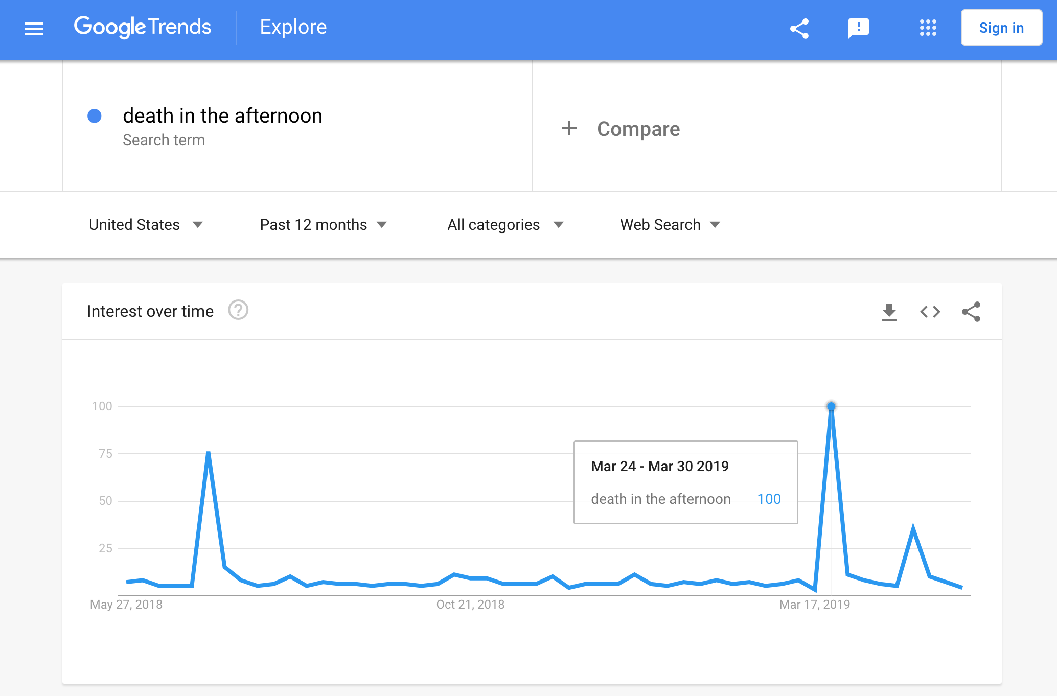
If we just isolate the clue to the subject “death in the afternoon”, we also see the spike:
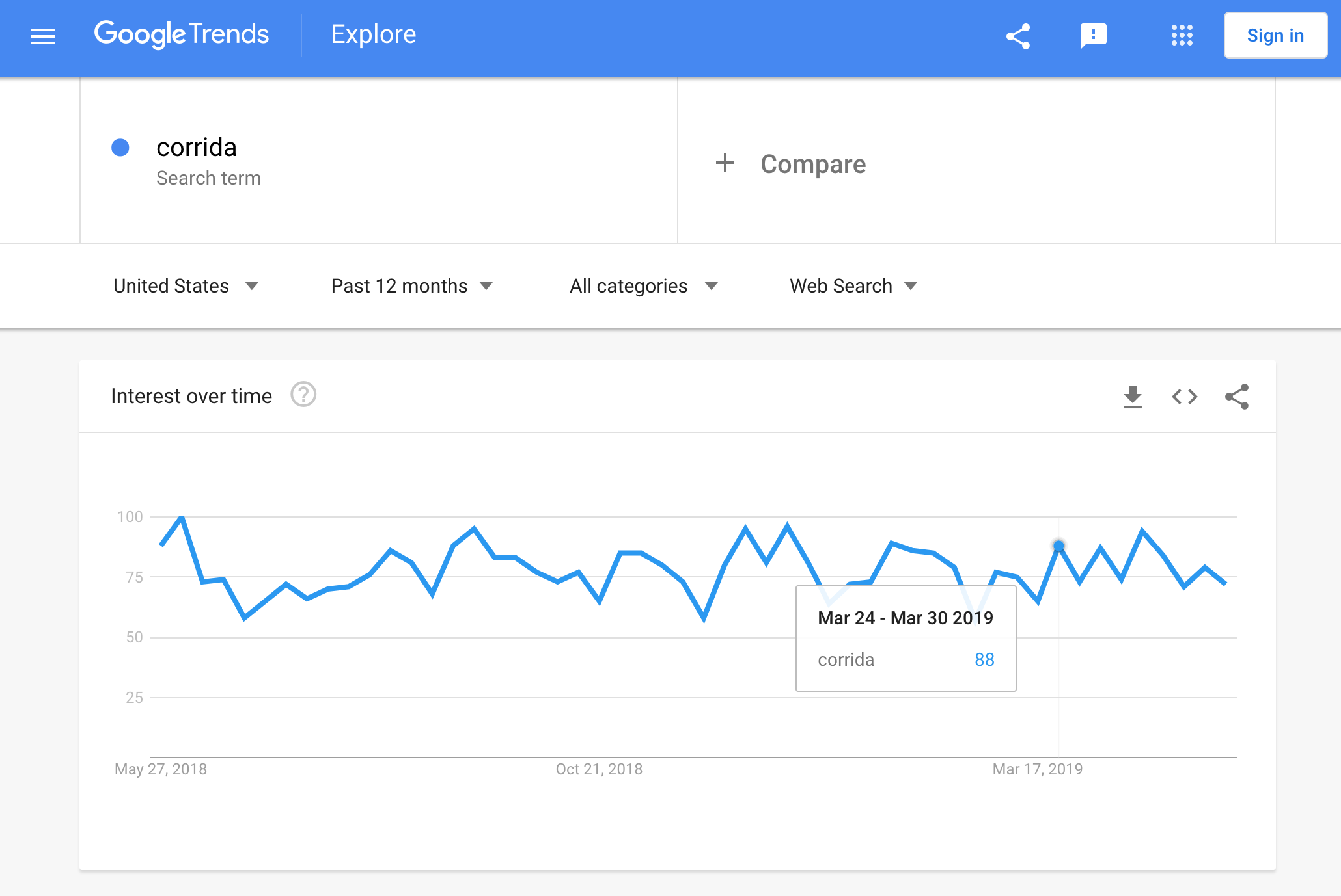
The subject of Hemingway’s book “Death in the Afternoon” is bullfighting. Since the setting was distinctly spanish, the answer here is “CORRIDA”. Looks like there is a visible spike for corrida on the same day among its typical search trends:
By default, Google Trends show weekly data in the UI. But we can use the Python package pytrends to get more granular data through Google’s API
from pytrends.request import TrendReq
import pandas as pd
import matplotlib.pyplot as plt

pytrends = TrendReq(hl='en-US', tz=360)
kw_list = ["death in the afternoon"]
pytrends.build_payload(kw_list, cat=0, timeframe='today 3-m', geo='', gprop='')

trend_df = pytrends.interest_over_time()
_ = trend_df.plot(figsize=(16,5))
_.set_title('Daily Google Search Trend Index', loc='left', fontdict={'fontweight':'extra bold'})
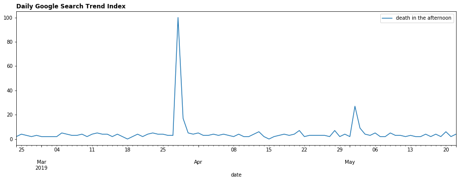
Quantifying Spike - How many people are cheating?
Can we quantify the spike? Yes - relatively. For reference, Google explains its index as:
Numbers represent search interest relative to the highest point on the chart for the given region and time. A value of 100 is the peak popularity for the term. A value of 50 means that the term is half as popular. A score of 0 means there was not enough data for this term.
So if the number of searches on a national scale remains constant, and a topic with 1,000 average searches sees a spike up to a peak of 10,000 searches, then we can expect the index to go from 10 to 100.
But what do we measure the spike to? It’s easy to see a spike for esoteric clues whose search trends might usually be low, but when it’s a relatively popular subject, we need a way to measure the uplift by defining a baseline. Look at this popular clue and its search trend:
54 Across: Issa of “Insecure”
The popularity of Issa Rae, star of Insecure and many other TV shows make it more difficult to spot the spike on 3/28. We’ll need a baseline. We can arbitrary decide on a baseline of 6 weeks and see what looks like with a few lines in Python:
from datetime import datetime, timedelta

def get_daily_trends(keyword, pytrends):
    kw_list = [keyword]
    pytrends.build_payload(kw_list, cat=0, timeframe='today 12-m', geo='', gprop='')
    trend_df = pytrends.interest_over_time()

    return trend_df

def calculate_uplift(trend_df, keyword, spike_week, baseline_window=6):
    baseline_week_start = datetime.strptime(spike_week, '%Y-%m-%d') - timedelta(weeks=baseline_window)
    baseline_week_end = datetime.strptime(spike_week, '%Y-%m-%d') - timedelta(weeks=1)

    baseline_average = trend_df[baseline_week_start:baseline_week_end][keyword].mean()
    spike_value = trend_df[spike_week:spike_week][keyword].values[0]

    return spike_value / baseline_average


keyword = 'Issa of "Insecure"'
issa_df = get_daily_trends(keyword, pytrends)
calculate_uplift(issa_df, keyword, '2019-03-24', 6)

>>> Uplift of 2.74x
Now I can calculate the difference between the crossword puzzle’s published date or week to determine a multiplier (or percent increase) over a period of time before.
| Index Change | Multiplier | % Increase |
|---|---|---|
| 50 -> 100 | 2x | 100% |
| 25 -> 100 | 4x | 200% |
| 10 -> 100 | 10x | 900% |
Evaluating an Entire Puzzle
Now I’m ready to apply my “cheating algorithm” to an entire puzzle. With my New York Times crossword subscription, I’m able to retrieve a JSON file of the puzzle, and I can iterate through the clues and search on Google Trends. For the March 28th puzzle, here’s a list of “tough” clues that received an increase amount of searches.
| Clue | Multiplier |
|---|---|
| 1A: Volunteer’s Offer | 2.34 |
| 2D: Subject of Hemingway’s “Death in the Afternoon” | 100 |
| 4D: Label on some packages of jerky | 99 |
| 9A: Nickname for Cleveland Browns fans | 50 |
| 23A: Down Under predator | 100 |
| 25D: Banned pollutants | 4.38 |
| 32A: Bonny miss | 2.52 |
| 54A: Issa of Insure | 1.88 |
| 55A: Boston Garden legend Bobby | 100 |
| 59D: Cocoon dwellers | 6 |
This quick analysis shows that yes, people are indeed cheating by Googling the clues for specific answers. What’s funny to me is that even a meta clue like 64 across that relates to the theme of the puzzle saw a 25x increase in searches:
64A: Request needed to understand four clues in this puzzle
Coming Up
In part 2 and 3 of this series, I’ll explore what kind of people are cheating with more Google Trend data, and how I might estimate puzzle difficulties just based on search volume. I’d assume easier puzzles on Monday would have less “cheat” compared to Saturday, but we’ll see!
-->